Smile Models

A trader or investor holding a portfolio of options or other derivatives based on a given underlying asset —be it cryptocurrency, an index, or a stock— needs a mid-volatility surface to accurately mark the portfolio to market at any point in time.

The volatility surface is a financial object that provides the volatility for any given expiry and strike price. This mid-volatility surface is derived from the bid and ask prices quoted in the options market using a smile model, which involves a fitting process and an interpolation across expiries.

Using bid/ask quotes directly to mark a derivatives portfolio is not feasible because different positions might require different volatilities—some should use bid volatility and others ask volatility. For complex derivatives that cannot be easily replicated with vanilla options, it becomes unclear whether to use bid or ask volatility.

Therefore, it is essential to construct a mid-volatility surface. This approach offers a consistent and unique view of the portfolio's value and associated risks.

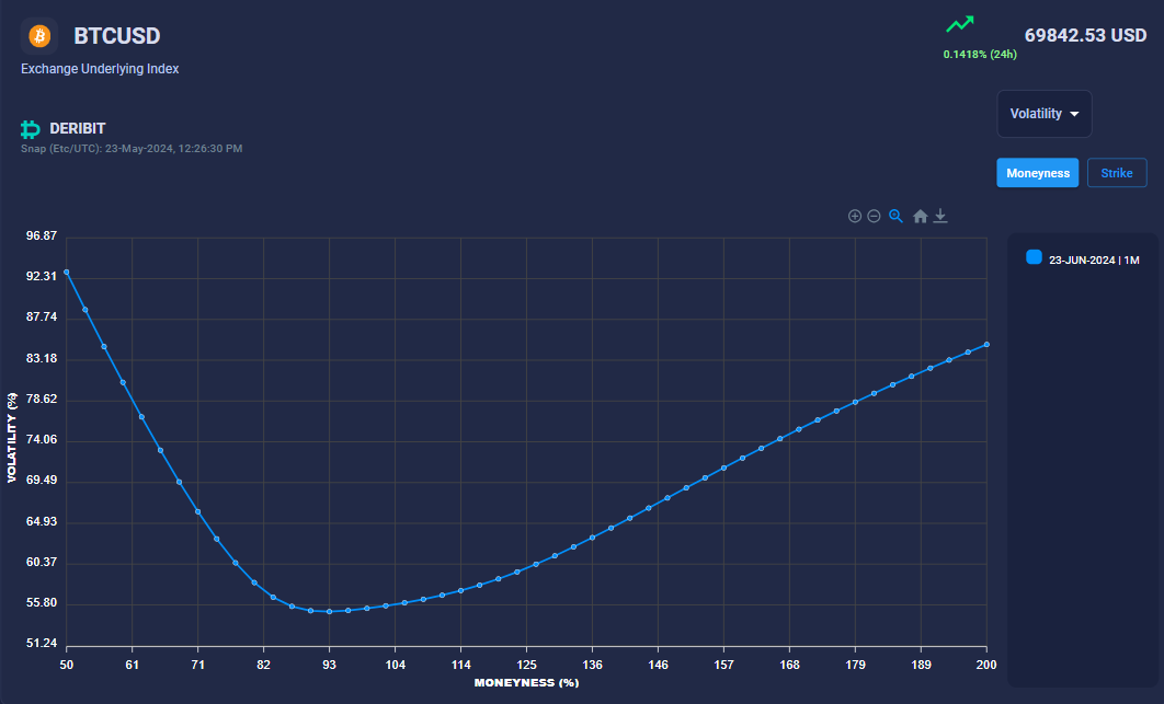
Introduction to the Volatility Smile

In financial markets, the volatility smile is a characteristic of the options market where implied volatility varies across different strikes. This behavior contradicts the assumptions of the Black-Scholes model, which presumes constant volatility across strikes. As a result, the Black-Scholes model often leads to pricing inaccuracies, particularly for deep in-the-money and out-of-the-money options.

Why Does the Volatility Smile Occur?

The volatility smile can be attributed to several market factors:

• Market sentiment and demand: High demand for out-of-the-money puts and calls can increase their prices and thus their implied volatilities.
• Stochastic nature of volatility: Volatility itself can be volatile and mean-reverting.
• Jump risk: Sudden jumps in asset prices, which are not accounted for in normal distributions used in simpler models.

Modeling the Volatility Smile

To account for the smile, several models have been developed. Here, we focus on two main types: the SABR and SVI models.

SABR Model

The SABR model is a popular choice for modeling options volatilities in the interest rate and equity derivatives markets. The model is particularly favored for its ability to capture the correct skewness and smile shape of the volatility surface as observed in market data. The model is derived from a stochastic diffusion of the underlying asset of the option.

The dynamics of the SABR model are described by the following stochastic differential equations (SDEs):

$$dS_t = \alpha S_t^\beta Z_t dW_t$$ $$dZ_t = \nu Z_t dB_t \:\;Z_0=1$$ $$\left\langle dW_t,dB_t\right\rangle =\rho dt$$

Where:

• $S_t$ is the forward price of the asset.
• $W_t$ is brownian motion driving the asset and $B_t$ the driver of the stochastic volatility.
• $Z_t$ is the normalised stochastic volatility factor.

The asset has a CEV (constant elasticity of variance model) like dynamic driven by the $\beta$ parameter. $\beta=1$ gives a log-normal diffusion and $\beta=0$ gives a normal diffusion. $\alpha$ is the CEV volatility.

The stochastic volatility has a log-normal diffusion with a volatility given by $\nu$. The asset and the stochastic volatility are correlated.

Let's provide some intuition on the SABR parameters:

• $\alpha$ controls the at-the-money (ATM) volatility and the overall level of the smile.
• $\rho$ governs the volatility skew, or equivalently, the slope of the smile around the ATM strike.
• $\nu$ determines the convexity of the smile.
• $\beta$ plays a dual role: it influences the relationship between the ATM volatility and the forward price while overlapping with $\rho$ to offer additional flexibility in controlling the skew.

The volatility surface is defined by the popular formula derived in the original SABR paper:

$$\sigma(T,K,S_0)=\frac{z}{ln(\frac{\sqrt{1-2\rho z+z^{2}}-\rho+z}{1-\rho})}\frac{\alpha}{S_m^{1-\beta}(1+\frac{(1-\beta)^{2}}{24}ln^{2}(\frac{S_0}{K})+\frac{(1-\beta)^{4}}{1920}ln^{4}(\frac{S_0}{K}))}(1+\\[10pt] (\frac{(1-\beta)^{2}}{24}\frac{\alpha^{2}}{S_m^{2(1-\beta)}}+\frac{1}{4}\frac{\rho\beta\nu\alpha}{S_m^{1-\beta}}+\frac{(2-3\rho^{2})}{24}\nu^{2})T)$$

where $S_m=\sqrt{S_0K}$ and $z=\frac{\nu}{\alpha}S_m^{1-\beta}ln(\frac{S_0}{K})$

This formula is an approximation of the implied volatility of the SABR diffusion

QSVI Model

The SVI model by Gatheral is another popular smile model. Unlike SABR, which is based on a stochastic volatility diffusion, the SVI model is a parametric representation of the option smile.

For a given expiry the volatility smile is given by the formula

$$\sigma^{2}(k)=a+b(k-m)+\sqrt{(k-m)^{2}+\gamma^{2}}$$

where k is the log-moneyness $k=ln(\frac{K}{S_0})$

Gatheral suggests a re-parametrisation of the model which is more intuitive

$$\begin{align*} \sigma_{ATM}^{2}= & a+b\left(-\rho m+\sqrt{m^{2}+\gamma^{2}}\right)\\ \sigma_{min}^{2}= & a+b\gamma\sqrt{1-\rho^{2}}\\ S_{ATM}= & \frac{b}{2\sigma_{ATM}}\left(\rho-\frac{m}{\sqrt{m^{2}+\gamma^{2}}}\right)\\ S_{L}= & b\left(\rho-1\right)\\ S_{R}= & b\left(1+\rho\right) \end{align*}$$

The new parameters have clear meanings:

• $\sigma_{ATM}$ is the at-the-money (ATM) volatility.
• $\sigma_{min}$ is the minimum volatility on the smile.
• $S_{ATM}$ is the smile slope at the ATM strike.
• $S_L$ is the asymptotic slope of the smile for low strikes.
• $S_R$ is the asymptotic slope of the smile for high strikes.

In our platform, we've developed an advanced extension of the SVI smile model to overcome its limitations and enhance its accuracy. While the SVI model, similar to the SABR model, includes parameters for ATM volatility, skew, and convexity around the ATM strike, it often struggles to fit both low and high strikes accurately due to its wing skew limitations. To address this, we've created a custom extension called the QSVI model. The QSVI model incorporates separate drivers for low and high strikes in addition to the standard parameters, allowing for a more precise fit across the entire range of strikes. This innovation provides traders with more reliable data and improved modeling capabilities, making our platform a superior choice for options and derivatives trading.

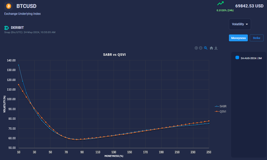
Below, we compare the QSVI smile and the SABR smile for the 3-month expiry, both fitted to the same market data. For a range of strikes around the ATM, both models produce similar volatilities. However, noticeable differences emerge on the far left and right wings. This discrepancy arises because there are no quotes for the far out-of-the-money (OTM) or in-the-money (ITM) strikes, and the extrapolation on the wings is driven solely by each model's parameterization. Additionally, SABR has fewer degrees of freedom compared to QSVI for the wings.

Fitting process

The smile fitting process is a delicate procedure that requires careful attention to the nuances of the options market data. It is essential to understand the specific market data we are trying to fit and adapt it accordingly to align with the smile model.

For options traded on exchanges, such as cryptocurrencies, equity stocks, or commodity assets, the data structure differs significantly from that of over-the-counter (OTC) options like FX options or interest rate options. Typically, exchange-traded options list a set of absolute strikes that change daily to reflect spot market movements. Additionally, the liquidity of option prices across expiries can vary widely and change over time. Some expiries may have only a few quoted strikes, while others may have many. Liquidity drops can cause certain expiries to disappear from the options quotes altogether. The bid/ask spread can also be inconsistent across strikes, leading to potential calendar or butterfly arbitrage opportunities within the smile.

OTC options, on the other hand, are generally simpler in this regard. They are typically quoted on a standard set of strikes across expiries and over time. The mid volatilities for OTC options are marked consistently and rarely imply arbitrage opportunities.

Options bid/ask data

This section will focus on BTCUSD options traded on exchanges such as Deribit and OKX. These exchanges provide a list of bid and ask prices for call and put options across various expiries and strikes at any given time. Typically, the exchanges quote options with daily, weekly, monthly, and quarterly expiries. Each time one of these expiries matures, the exchange introduces a new one to replace it. For example, there is a 1-day expiry every day and a 1-week expiry every Friday.

The range of quoted strikes is designed to cover a meaningful delta range, with granularity based on the asset's typical daily movement.

Cleaning of bid/ask data

The bid/ask prices are not always consistent across expiries and strikes, meaning they may not be arbitrage-free. Therefore, we clean the bid/ask price data before fitting it.

Here is a brief description of the steps we take to clean the data:

• Retain only out-of-the-money prices: puts for strikes below the forward price and calls for strikes above the forward price.
• Remove all bid/ask pairs where the bid-ask spread exceeds a certain threshold, typically when the spread divided by the forward price is above 6% (we use this valued based on the analysis of the historical data of the bid-ask spreads).
• Eliminate all call or put prices that are not monotonic in strike.
• Remove all successive call or put prices that imply a digital option price above 1.
• Remove all successive call or put prices that imply a butterfly spread price below 0.

We apply these steps to both the bid and ask prices independently.

After that, we obtain a set of arbitrage-free bid/ask prices. For a given strike, it is possible to have only a bid or only an ask, either because the exchange did not quote both or because the cleaning process removed one of them.

Finally, we calculate the implied volatilities for each bid and ask price and fit the model to this data.

Calibration

Calibration of the smile model involves adjusting the model parameters to ensure that the model prices align with the observed market prices. This process begins with cleaning the data and computing the implied volatilities from the bid/ask prices. We then fit a unique set of model parameters for each expiry. Since shorter expiries have a narrower range of strikes, and our goal is to maintain stable wings over time, we start by independently fitting expiries with a sufficiently large strike coverage.

To achieve this, we minimize the distance to the mid volatility as well as the bid and ask volatilities, applying a heavier penalty for deviations from the bid/ask prices than from the mid. Additionally, we incorporate a calendar arbitrage penalty to prevent the variance of the current slice from being lower than that of the previous slice.

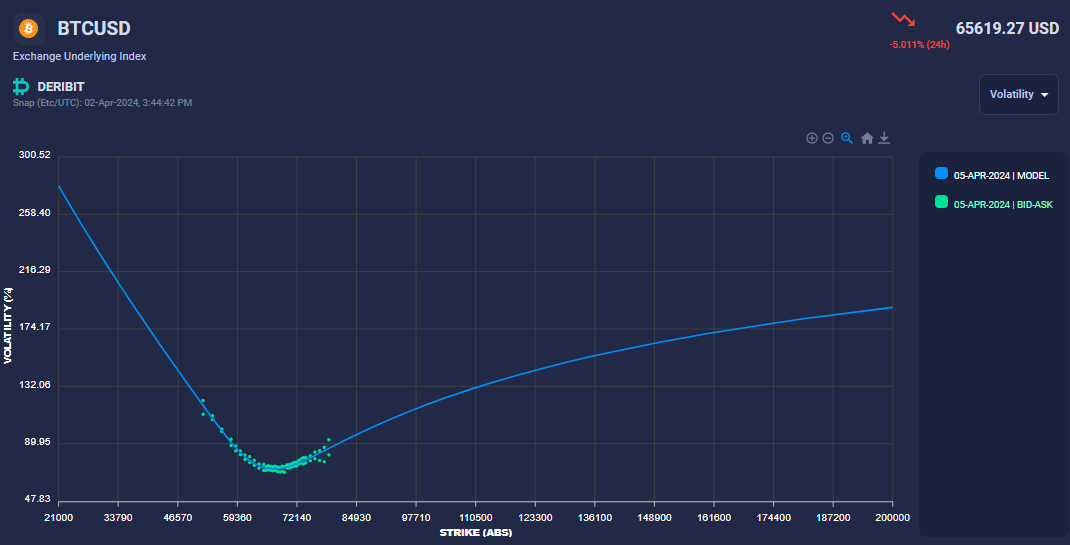
After fitting these longer expiries, we proceed to fit the shorter expiries. For shorter expiries, we impose an additional constraint on the smile wings, keeping them close to the previous slice's wings. This is necessary because short expiries often lack quotes for low and high strikes, providing insufficient data for the smile model to determine a unique solution. As shown in the first picture below, short expiries typically have bid/ask prices within a narrow range around the ATM, unlike longer expiries. This is because, for short expiries, options with strikes far from ATM have little chance of moving close to ATM by expiry, so the market does not quote strikes far from ATM.

The lack of information on the far wings poses a challenge for fitting the model, as the optimizer can easily become trapped in local minima far from the optimal solution. Therefore, we anchor the short expiry wings to the long expiry wings, which have more quotes on the far wings.

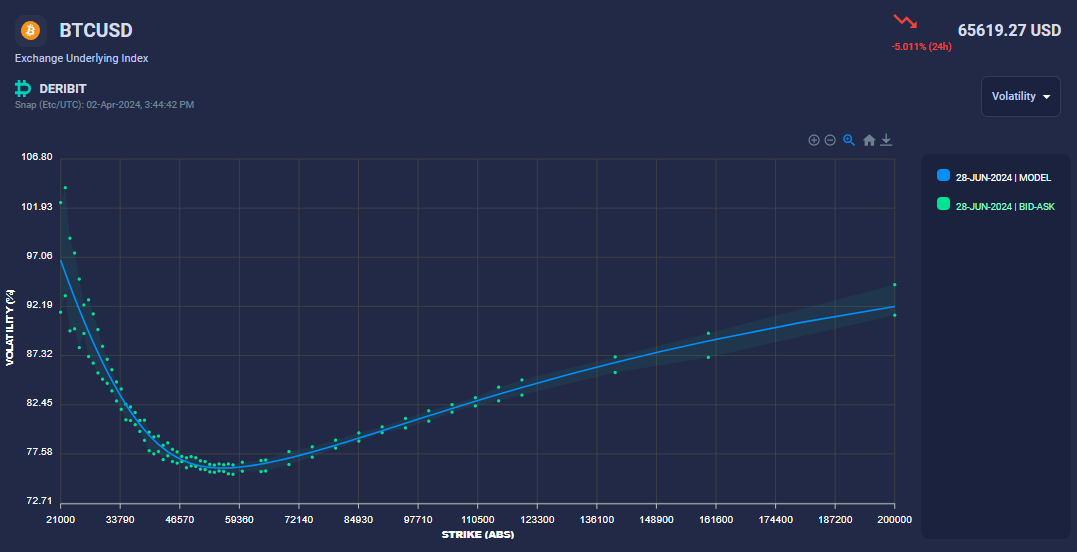
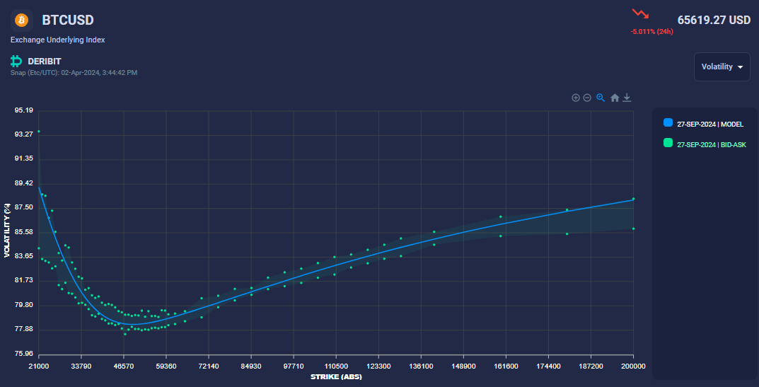
Below, we show three expiries: 5Apr24, 28Jun24, and 27Sep24. For the longer expiries, the bid-ask spreads are wider and more noisy, which can sometimes induce arbitrages. These arbitrages are addressed through the data cleaning process described above.

---